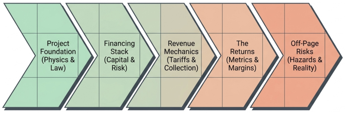
Part 1	The Project First, the Spreadsheet Second	What am I actually looking at?
Part 2	The Financing Stack	How is this being paid for – and is it realistic?
Part 3	Revenue, Tariffs and What You Will Actually Collect	Will the money actually come in?
Part 4	Reading the Returns	What does the model claim to deliver – and for whom?
Part 5	The Risks the Model Leaves Off the Page	What could quietly sink this project?

PART 1 – The Project First, the Spreadsheet Second

A hydropower financial model is only as good as the project it describes. Before opening a single spreadsheet, it makes sense to spend time understanding what has been built, where it is, what it generates, who owns it, and – critically – at what stage of legal development it sits. Numbers in a model mean nothing if the project they represent is missing a licence or three years from breaking ground.

This part covers how to extract and verify the physical and legal fundamentals that every financial model should be anchored to.

1.1 The Salient Features – Your Project Checklist

Every hydropower project has a set of engineering parameters that determine its financial character. These are not decorative disclosures. They are the load-bearing walls of the entire model. Check every one of them.

Installed Capacity (MW)	Total nameplate generation capacity in megawatts	Sets the ceiling on revenue; determines royalty base
Design Head (metres)	The vertical drop of water between intake and turbine	Higher head = greater efficiency; Pelton turbines above ~300m, Francis below
Powerhouse Type	Surface, underground, or semi-underground	Underground adds significant civil cost but reduces environmental impact and risk
Annual Energy Generation (GWh)	Gross energy produced per year	Primary driver of revenue; verify against hydrology studies
Firm Peaking Capacity (MW × hours)	Guaranteed dispatchable power at peak times	Determines premium tariff eligibility and grid value
Plant Load Factor / Capacity Factor (%)	Ratio of actual energy to theoretical maximum	See equation below – critical for revenue validation
Basin and River	Which river system, which catchment	Determines hydrology, sediment, GLOF and cascade risk
Access Road	Completed, under construction, or planned	Affects construction cost and timeline certainty
Construction Period	Number of months from financial close to COD	Every extra month adds interest during construction (IDC)
Licence Period	Total years of operating right granted	Determines the revenue horizon; check when it starts
Total Project Cost	Overnight cost excluding financing charges	Base for all cost ratios and sensitivity analysis
Developer / SPV	Legal entity holding the project	Ownership structure affects tax treatment and repatriation
Promoter Mix	Government, institutional, public float	Affects equity call risk and IPO dependency

Hydroelectric Turbines: Pelton vs. Francis

1. Pelton Turbine: An impulse turbine designed for high-head (steep drop) and low-flow water conditions. It utilizes high-velocity water jets striking spoon-shaped buckets on a wheel to generate mechanical energy entirely under atmospheric pressure.
2. Francis Turbine: A reaction turbine optimized for medium to low-head and high-flow conditions. Unlike the Pelton, it operates completely submerged in water, utilizing both pressure and kinetic energy as the water flows radially inward through the runner blades.

Powerhouse Configurations

1. Surface Powerhouse: The most common and cost-effective configuration, where the generating equipment is housed in a structure built entirely above ground at the base of the water source, offering easy accessibility for maintenance.
2. Underground Powerhouse: Excavated deep within a mountain or below ground level, this type is used when surface space is limited, geological conditions permit, or environmental and topographical constraints require protecting the facility from external hazards.
3. Semi-Underground Powerhouse: A hybrid design where a significant portion of the structure is excavated below ground level while the upper section remains exposed, balancing architectural protection with ease of construction and ventilation.

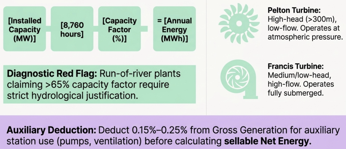
Converting Megawatts to Megawatt-Hours: The Essential Equation

One of the most common errors in model review is accepting the annual energy figure without checking it. The conversion from installed capacity to annual energy is governed by a single relationship:

Annual Energy Calculation Annual Energy (MWh) = Installed Capacity (MW) × 8,760 hours/year × Capacity Factor (%)  Example: A 100 MW plant with a 50% capacity factor produces: 100 × 8,760 × 0.50 = 438,000 MWh = 438 GWh per year  For a high-head peaking hydropower project in a mountain basin, typical capacity factors range from 45% to 60% depending on hydrology, reservoir storage, and seasonal flow patterns. A run-of-river plant on a snow-fed river may range from 35% to 50%.  Red flag: If the model’s stated energy figure implies a capacity factor above 65% for a run-of-river plant, demand justification from the hydrological study.

Auxiliary Consumption: Gross vs. Net Energy

The energy figure in most tariff agreements – and therefore in the revenue calculation – is net energy: the amount delivered to the grid after the plant’s own internal consumption has been deducted.

An underground powerhouse running dewatering pumps, ventilation fans, lighting systems, control equipment, and transformer losses will typically consume 0.15% to 0.25% of gross generation internally. This is called auxiliary consumption or station use. It sounds small but on a large plant it can represent several gigawatt-hours per year that the model should not count as sellable revenue.

Auxiliary Consumption Check Net Sellable Energy = Gross Generation × (1 − Auxiliary Consumption %)  For a 1,000 GWh/year plant at 0.2% auxiliary consumption: Net Energy = 1,000 × (1 − 0.002) = 998 GWh  This difference (~2 GWh) is modest at 0.2%, but a model that sets auxiliary consumption to zero while the engineering report assumes an underground powerhouse is inconsistent and should be corrected before any external use.

1.2 The Licence and Agreement Timeline – Where Dates Come From

The financial model’s key dates – financial close, construction start, commercial operation date (COD) – are not freely chosen by the project developer. They are determined by a chain of legal instruments, each of which must be in place before the next one can be executed. Understanding this chain is essential to testing whether the timeline in a model is realistic.

Document / Licence	What It Does	Financial Significance
Survey Licence	Authorises investigation and feasibility studies on a river reach	Starting point; without this, no legal right to develop exists
Generation Licence	Grants the right to generate electricity from the project	Required before PPA can be signed; lenders will not commit without it
Project Development Agreement (PDA)	Government agreement confirming project support, land rights, and fiscal terms	Locks in royalty rates, tax concessions, and government equity obligation
Environmental Impact Assessment (EIA) Approval	Regulatory clearance for construction	Construction cannot begin – and lenders will not disburse – without this
Power Purchase Agreement (PPA)	Offtake contract with the buying utility (tariff, volume, duration, payment terms)	The single most important revenue document; its terms flow directly into the model; and the concession licence clock
Transmission / Wheeling Agreement	Rights to evacuate power to the grid	Without this, energy cannot be sold regardless of generation
Financial Close (Loan Agreement + Equity Subscription)	All financing committed and conditions precedent satisfied	The model’s construction start date cannot precede this
Sponsors / Shareholders Agreement	Governs equity contributions, governance, and dispute resolution between promoters	Affects equity call timing and modelled equity drawdown schedule
Commercial Operation Date (COD)	Certified start of full commercial generation	Triggers tariff payments, royalty obligations

The chain matters because each document, when executed, sets or constrains the next date. A model that shows financial close in Month 6 when the EIA has not yet been granted is not conservative – it is wrong. When reviewing a model, ask: which of these documents are in place today, which are in process, and which have not yet been initiated?

The Timeline Stress Test For each undone document, ask: what is the realistic best-case time to completion? Add those up. If the sum pushes financial close beyond the model’s assumed date, every subsequent date in the model is also wrong – and every interest-during-construction figure is understated.

1.3 What Financial Close Actually Means

Financial close is the moment at which all lenders and equity investors have signed their agreements, all conditions precedent (CPs) have been satisfied, and the project can begin drawing down funds. It is a legal event, not just a financial one.

Typical conditions precedent that must be satisfied before financial close include: signed PPA, signed generation licence, EIA approval, land acquisition completion, financial model approval by all lenders, insurance placement, independent engineer appointment, and legal opinions from project lawyers. In practice, negotiating and satisfying all of these simultaneously – with multiple lenders, a government counterparty, and an offtaker – takes far longer than developers estimate.

Key Takeaway – Part 1 Never review the numbers before you have verified the project’s legal and documentary status. A model projecting COD in 2030 means nothing if there is no signed PPA, no EIA, and no confirmed financing. The most important question a reviewer can ask is not ‘what does the model show?’ but ‘what has actually been signed?’

PART 2 – The Financing Stack

A hydropower project is almost never built with equity alone. The combination of sources – debt, equity, and sometimes concessional public finance – determines the cost of capital, the risk distribution between stakeholders, and ultimately whether the project can survive the inevitable moments when revenue disappoints or costs overrun. Part 2 examines how the financing structure should be assembled, what each component means, and where financial models most commonly go wrong.

2.1 The Debt-Equity Ratio – The Architecture of Risk

The debt-equity ratio (also called the leverage ratio or gearing) is the single most influential structural parameter in a hydropower financial model. It determines how much of the project is funded by debt – which must be repaid with interest – and how much by equity – which bears the residual risk.

Debt-Equity Ratio Equation Debt-Equity Ratio = Total Debt : Total Equity  Example: A 70:30 ratio means 70% of total project cost is funded by debt and 30% by equity.  For a project costing USD 1,500M:   Debt = USD 1,050M   Equity = USD 450M  Typical ranges for hydropower: 60:40 (conservative) to 80:20 (highly leveraged). Higher leverage amplifies equity returns but reduces the cushion available to service debt if revenue falls short.

A higher debt ratio (more leverage) benefits equity investors in good times because they receive the upside on a smaller invested base. However, it also concentrates risk on the project’s ability to generate sufficient cash flow to service the debt every year – which is measured by the Debt Service Coverage Ratio (DSCR), discussed in Part 4.

Domestic vs. International Debt

In most emerging-market hydropower projects, the debt stack is a blend of domestic commercial bank loans and international concessional finance. These two types of debt have fundamentally different cost profiles, tenors, and conditions attached to them.

Debt Type	Typical Interest Rate	Typical Tenor	Conditions
Domestic commercial bank	10–12% per annum	10–15 years	Few conditions; faster to close; limited by bank exposure limits
Government pension / provident funds	8–10% per annum (administered rate)	15–30 years	Subject to regulatory approval; requires government on-lending framework
Multilateral (World Bank, ADB, IFC)	0.5–2.5% per annum	25–40 years	Environmental, social, procurement standards; downstream riparian consent may be required
Bilateral concessional (JICA, KfW, etc.)	0.1–1.5% per annum	30–40 years	Tied procurement in some cases; slower processing
Export credit agencies	3–5% per annum	15–20 years	Usually tied to exporting-country equipment supply

The cost gap between domestic commercial debt (say 10%) and multilateral concessional debt (say 1%) on a USD 1 billion loan is enormous. Over 25 years, the difference in total interest payments can exceed the original equity invested. This is why access to concessional financing is often the difference between a financially viable project and one that cannot generate adequate returns.

Concessional Government On-Lending: Why It Exists and Why It Is Risky to Assume

In many developing countries, governments act as financial intermediaries: they borrow cheaply from pension funds, development banks, or their own budget, and then on-lend those funds to state-sponsored infrastructure projects at a subsidised rate through a Subsidiary Loan Agreement (SLA). The government absorbs the spread between its own borrowing cost and the rate charged to the project.

This mechanism – variously called viability gap funding, concessional on-lending, or a subsidised SLA – can transform the economics of a project that would otherwise be unviable at market rates. However, it creates a critical assumption risk in any financial model: it must be formally confirmed by the government authority with the power to commit public funds.

Critical Check – Concessional Loan Assumption If a financial model includes a below-market government loan (e.g., at 1–3% over 25+ years), verify: 1. Has a formal government decision or term sheet been issued? 2. Which ministry or fund is the source – and do they have legal authority to commit? 3. What are the conditions – does it require project milestones, foreign co-financing, or regulatory approvals?  If the answer to any of these is ‘not yet confirmed,’ run the model again replacing the concessional loan with a domestic commercial rate. If the project fails under that scenario, the concessional loan is not a financing assumption – it is the project’s entire financial case.

The Foreign Currency Component

Large hydropower projects procure turbines, generators, transformers, and often engineering and construction services from international suppliers. This creates a foreign currency (forex) component in total project cost – typically 30–50% of overnight cost for a large scheme. This matters for two reasons.

First, the project’s total cost in local currency terms depends on the exchange rate at the time of procurement. If the local currency has depreciated since the model was built, actual cost in local currency will be higher than modelled. Second, if any debt is denominated in foreign currency, every payment of principal and interest carries exchange rate risk – the loan gets more expensive in local currency terms every year the currency depreciates.

Foreign Exchange Depreciation Check Step 1: Find the model’s assumed annual depreciation rate for local currency vs. USD (or relevant hard currency). Step 2: Look up actual historical depreciation over the last 10–15 years for the country. Step 3: If the model uses a rate materially below the historical average, run a sensitivity:  Corrected FX Depreciation Impact on Revenue (simplified): If 35% of costs are USD-linked and the model assumes 2.5% depreciation but history shows 4.5%: Additional annual cost escalation ≈ 35% × (4.5% − 2.5%) = 0.7% of total cost per year  Over 25 years this compounds significantly. Always stress-test at the historical average rate.

2.2 Insurance – The Most Underestimated Line in the Model

Insurance for a large hydropower plant is not a standard property insurance question. These are complex, high-value assets in remote, physically hazardous locations with long construction periods, limited access for emergency response, and exposure to natural hazards that most commercial insurers handle only through specialist reinsurance markets.

A comprehensive insurance programme for a large hydropower project typically includes:

• Construction All-Risks / Erection All-Risks (CAR/EAR): Covers physical damage during construction to civil structures, electromechanical equipment, and third-party liability. This is time-limited to the construction period.
• Operational Property Damage: Covers the replacement cost of the plant against fire, flood, mechanical breakdown, and other insured perils.
• Business Interruption (also called Loss of Revenue or Loss of Profits): Covers revenue lost during a period when the plant cannot generate due to an insured event. This is the most financially critical cover for project finance lenders.
• Third-Party Liability: Covers claims from downstream communities or infrastructure affected by project operations or failure.
• Natural Catastrophe Riders: In seismically active or glacially exposed basins, specialist covers or exclusion carve-outs must be negotiated specifically.

Insurance Sizing Benchmark For a large hydropower plant in a mountainous, high-risk geography:  Property Damage: 0.4–0.8% of insured replacement value per year Business Interruption: 0.15–0.25% of annual revenue per year Third-Party & other: 0.05–0.1% of replacement value per year Total indicative range: 0.6–1.2% of insured value per year  If the model uses a figure below 0.5% of total project cost as total annual insurance premium, it is likely underestimating. Obtain at least indicative quotes from a specialist infrastructure insurance broker before finalising the model.

The Domestic Insurance Market Limitation

In many developing countries, the domestic insurance market does not have the balance sheet capacity to underwrite multi-hundred-million dollar infrastructure risks. This means that even if a local insurer issues the policy, the actual risk is passed to international reinsurance markets through reinsurance treaties. The practical consequence is that the premium pricing will be driven by international market rates for comparable Himalayan or tropical large hydro risks – not by domestic market competition. Models that assume domestic-market insurance rates for a project that will require London-market reinsurance will systematically understate the cost.

2.3 Operation & Maintenance Cost

Operation and maintenance (O&M) cost is typically modelled as a percentage of total project cost (or ‘build cost’), escalated by an inflation assumption each year. For a well-maintained large hydropower plant, the base O&M rate is usually in the range of 0.25% to 0.40% of build cost per year, with higher rates applicable in the first decade (commissioning and initial maintenance) and later years (aging equipment).

O&M Cost Check Annual O&M Cost = Build Cost × O&M Rate  For a USD 1,200M project at 0.3%: O&M = USD 3.6M/year in base year Escalated at 3.5% per year: by Year 20, O&M ≈ USD 7.2M/year  Key questions: 1. Does the O&M rate include major equipment overhaul costs, or are those separately modelled as lump-sum replacement capex? 2. Is the inflation rate applied to O&M consistent with local construction/labour cost inflation – not just general CPI? 3. In high-sediment river basins, does the O&M provision include a specific sediment management reserve?

2.4 Weighted Average Cost of Capital (WACC)

The WACC is the blended cost of all capital used to finance the project, weighted by each source’s share of total funding. It is used both as the hurdle rate for project viability and as the discount rate in NPV calculations.

WACC Equation WACC = (Equity Weight × Cost of Equity) + (Debt Weight × Cost of Debt × (1 − Tax Rate))  Example:   Equity: 30% of capital at 14% required return   Debt: 70% of capital at 8% interest, tax rate 20%  WACC = (0.30 × 14%) + (0.70 × 8% × (1 − 0.20))      = 4.2% + 4.48%      = 8.68%  The debt cost is tax-adjusted because interest payments are usually tax-deductible, reducing the effective cost of debt. Note: if the project has a long tax holiday (e.g., 15 years of zero tax), the tax shield does not apply during that period and WACC is higher in early years.

WACC is highly sensitive to the cost of each component. A model that includes a heavily subsidised concessional loan at 1.5% will show a dramatically lower WACC than the same project financed at commercial rates. When that subsidised loan is uncertain, the WACC – and every NPV and IRR figure derived from it – is also uncertain.

2.5 Dividend Payout and Lender Covenants

Many financial models for infrastructure projects show a 100% dividend payout – meaning all profits after tax are distributed to shareholders each year. This is financially convenient for equity investors but creates a fundamental conflict with how sophisticated project finance lenders structure their loans.

Standard project finance lending covenants typically include:

• Debt Service Reserve Account (DSRA): A cash account funded to 6–12 months of forward debt service obligations. This must be funded before any dividend can be paid.
• Cash Sweep: A mandatory prepayment mechanism where a percentage of excess cash flow (after debt service) is used to accelerate debt repayment. This reduces the free cash available for dividends.
• Restricted Payment Test: A test applied before any dividend declaration that requires the DSCR to be above a specified minimum threshold (typically 1.15x to 1.25x) on a trailing and projected basis. If the project is performing below this level, dividends are blocked.

Dividend Payout vs. Lender Requirements A model showing 100% dividend payout effectively means the project distributes every dollar of surplus to equity holders, leaving nothing in reserve for debt protection. When such a model is presented to lenders, they will typically require:  1. A DSRA to be funded at financial close (reducing available equity return by that amount upfront) 2. A cash sweep reducing annual free cash flow 3. A restricted payment test that will block dividends in weaker years  The impact on equity IRR is modest in good scenarios (0.3–0.7% reduction) but significant in stress scenarios where dividends are blocked for multiple consecutive years.

Key Takeaway – Part 2 The financing structure is not a background assumption – it is the project’s financial DNA. A concessional loan that is not confirmed, an insurance figure that is 5× too low, or a dividend assumption that conflicts with lender covenants each has the power to change the project from viable to unviable. Review each line of the financing stack with the same rigour as the revenue projections.

PART 3 – Revenue, Tariffs and What You Will Actually Collect

Revenue in a hydropower model looks deceptively simple: energy generated multiplied by tariff per unit. In practice, the revenue line is where most of the risk lives. The tariff might be wrong. The energy might not be dispatched. The offtaker might not pay. The escalation stops. A charge you did not expect reduces your net receipt. This part works through each dimension of the revenue calculation.

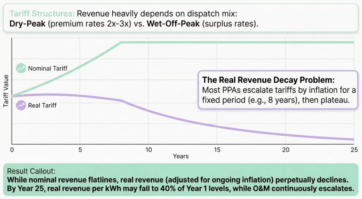
3.1 The Tariff Structure

Electricity tariffs for large hydropower projects in regulated markets are not freely negotiated to market clearing prices. They are determined through a combination of regulatory frameworks, bilateral PPA negotiations, and government policy. A typical tariff schedule for a peaking hydropower project distinguishes between:

Tariff Component	When It Applies	Typical Basis
Dry-Season Peak Tariff	Low-flow months; peak demand periods	Highest rate – 2× to 3× wet-season off-peak
Dry-Season Off-Peak Tariff	Low-flow months; off-peak demand periods	Intermediate rate
Wet-Season Tariff (all periods)	High-flow months; system surplus common	Lowest rate – reflects market surplus condition
Capacity Payment (if applicable)	Fixed monthly payment per MW of firm capacity	Compensates for availability regardless of dispatch

The split between dry-season and wet-season generation – and the relative volumes of peak vs. off-peak within each season – is therefore a critical revenue driver. A project that generates 60% of its energy in the wet season at low tariffs will have a very different revenue profile from one that stores and dispatches primarily in the dry season at premium rates.

Revenue Calculation Check Annual Revenue = Σ (Energy in period × Tariff for that period)  Example (simplified four-period model):   Dry-Peak:     150 GWh × Tariff A = Revenue A   Dry-Off-Peak: 120 GWh × Tariff B = Revenue B   Wet-Peak:     200 GWh × Tariff C = Revenue C   Wet-Off-Peak: 530 GWh × Tariff D = Revenue D   Total: 1,000 GWh, Revenue = A+B+C+D  Verify: (i) that the energy split between periods is consistent with the hydrological study, and (ii) that the tariffs applied match the signed or draft PPA.

3.2 PPA Escalation and the Real Revenue Decay Problem

Most power purchase agreements for large infrastructure projects include a tariff escalation clause – a percentage increase applied to the base tariff each year to compensate for inflation. A typical clause might specify 3% per annum for the first 8 years, after which the tariff remains flat in nominal terms for the remainder of the concession period.

This structure creates a revenue profile that rises in the early years and then plateaus. What the model often does not make visible is what happens in real terms (i.e., after adjusting for inflation): once escalation stops, real revenue begins to decline permanently.

Real Revenue Decay Illustration Assume: Base tariff = 10 units/kWh; Escalation = 3%/yr for 8 years; Inflation = 5%/yr throughout  Year 1: Nominal tariff = 10.00; Real tariff (base year) = 10.00 Year 8: Nominal tariff = 12.67; Real tariff = 12.67 / (1.05^7) = 9.08 (already eroding) Year 15: Nominal tariff = 12.67 (flat); Real tariff = 12.67 / (1.05^14) = 6.40 Year 25: Nominal tariff = 12.67 (flat); Real tariff = 12.67 / (1.05^24) = 3.96  By Year 25, real revenue per kWh has fallen to 40% of the Year 1 level. Meanwhile O&M costs, staff costs, and royalties continue escalating with inflation. The project’s real margin narrows every year post-escalation cutoff.

This is not necessarily a fatal problem – many projects are designed with sufficient early-year cash generation to repay debt before the real revenue decline becomes severe. However, it must be visible in the model, and the DSCR profile in later years must be examined carefully.

3.3 Take-and-Pay vs. Take-or-Pay – The Offtake Risk Question

The payment obligation in a PPA is one of the most important – and most contested – terms in any hydropower agreement. The distinction between the two main structures is fundamental:

Structure	Offtaker’s Obligation	Risk Profile for Project
Take-and-Pay	Pay for energy only if dispatched; no payment if grid does not call for power	Project bears dispatch risk; revenue falls in surplus periods
Take-or-Pay	Pay for contracted volume whether dispatched or not; a ‘deemed generation’ payment if not called	Project bears availability risk only; revenue is more predictable
Capacity Payment (hybrid)	Fixed monthly payment for making capacity available, plus energy payment for dispatched units	Best for lenders; separates availability from dispatch revenue

In markets where grid surplus is structurally growing – as more generation capacity is added each year – the distinction becomes more financially significant over time. A project that came online in a supply-short market under take-and-pay terms may face serious dispatch curtailment a decade later when the grid is oversupplied.

Critical Check – Offtake Structure Identify clearly whether the PPA is take-and-pay or take-or-pay. If it is take-and-pay: 1. Model a dispatch curtailment scenario – what does revenue look like if 20–30% of wet-season energy is not called? 2. Consider the projected supply-demand balance for the grid in Year 10 and Year 20 of the project’s life – is dispatch guarantee economically sustainable for the offtaker? 3. If the offtaker is a single public utility, track whether there are policy signals of intent to renegotiate take-and-pay obligations.

3.4 Wheeling Charges – The Hidden Revenue Deduction

When a hydropower project delivers electricity to the national grid through transmission infrastructure owned by a third party (such as a separate state-owned transmission company or grid operator), it may be required to pay a wheeling charge – essentially a transmission access fee. Wheeling charges are deducted from revenue before the project receives its net tariff income.

Wheeling charge frameworks vary significantly by country and regulatory regime. A well-designed framework distinguishes between:

• Fixed Capacity Charge: A monthly or annual payment per MW of contracted transmission capacity, regardless of how much energy flows. This compensates the transmission owner for building and maintaining the infrastructure.
• Variable Energy Charge: A per-kWh payment based on actual energy transmitted. This reflects the marginal cost of transmission use.

From a project finance perspective, the risk in wheeling charges lies in regulatory uncertainty – particularly in markets where the framework is still being designed. If the charge is set after the PPA is signed, the project has no ability to pass it through unless the PPA includes an explicit transmission cost pass-through provision.

Wheeling Charge Risk If the wheeling charge framework is not finalised at the time of model preparation, the model should: 1. State clearly that the wheeling charge is assumed, not confirmed 2. Show a sensitivity for a 20% and 50% increase in the wheeling charge 3. Identify whether the PPA includes a transmission cost pass-through clause  If a fixed capacity component is later added to a model that only assumed a variable energy charge, the effective revenue reduction can be material – particularly in years of low dispatch.

3.5 Royalties – The Government’s Share of Revenue

In most countries with public ownership of water resources, hydropower developers are required to pay royalties to the government as compensation for using a public natural resource. Royalty structures typically combine a capacity-based component (paid per kilowatt of installed capacity per year) and an energy-based or revenue-based component (paid as a percentage of energy revenue).

Royalty rates commonly change over the licence period. A project in its first 15 years – when it is repaying debt and delivering returns to investors – typically pays a lower rate than in the later years when the debt is retired and cash flows are stronger. This design reflects the policy intention of making projects viable in early years while increasing the government’s share over time.

Royalty Timeline – What to Verify Check the royalty rates in the model against the current regulatory schedule and the Project Development Agreement: 1. Are capacity royalties correct for Years 1–15 and Years 16+? 2. Are revenue/energy royalties at the right percentage? 3. Are royalties calculated on gross revenue or net-of-wheeling revenue? 4. Is the royalty base MW consistent with licensed capacity (not just installed capacity if different)?  A 2× error in capacity royalty rates – applying the Year 16+ rate to Year 1 – can overstate royalty cost by hundreds of millions over the project life.

3.6 Tax Treatment

Hydropower projects in developing countries typically receive structured tax concessions to encourage investment in long-gestation, capital-intensive infrastructure. A common structure includes: a full tax exemption for an initial period (often 10–15 years), followed by a reduced rate for a transitional period, followed by the full corporate tax rate for the remaining concession life.

The financial model must apply this schedule precisely, as the income tax line is one of the largest cash outflows in the post-exemption years. Additionally, some jurisdictions allow accelerated depreciation during the exemption period – even though no tax is paid, the depreciation builds a tax asset that reduces future liability. Whether this is correctly modelled affects the post-tax cash flow in transition years significantly.

Key Takeaway – Part 3 Revenue in a hydropower model is not a single number – it is the product of four moving parts: energy volume, tariff structure, escalation trajectory, and offtake certainty. Each of these can disappoint. The model should show you what happens to revenue when any of them does. If it only shows the optimistic case, it is incomplete.

PART 4 – Reading the Returns

A financial model typically produces several different return metrics, each telling a different part of the story. Project IRR, equity IRR, government IRR, DSCR, payback period, levelised cost of energy – these are not interchangeable. Each answers a different question, and understanding the difference between them is essential for evaluating whether a project is truly viable or simply dressed up to look that way.

4.1 The Internal Rate of Return (IRR) – Three Numbers, Three Stories

The IRR is the discount rate at which the net present value (NPV) of all cash flows – in and out – equals zero. It is the single number most commonly used to summarise a project’s return. But for a hydropower project with multiple categories of investor, there are at least three distinct IRRs, each calculated on a different set of cash flows.

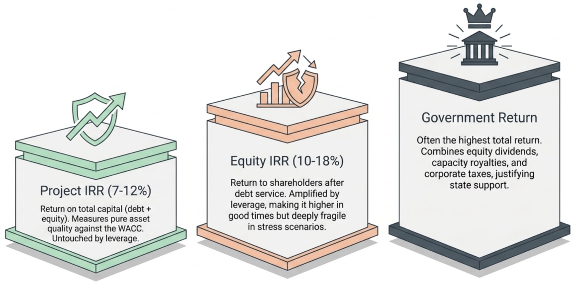
Project IRR (also called Unleveraged IRR or All-Equity IRR)

The Project IRR calculates the return on the total capital invested in the project – debt and equity combined – before any financing costs. It measures the return generated by the assets themselves, independent of how they are funded. This is the most stable metric because it is not affected by the financing structure.

Project IRR Cash flows used: Total investment (negative) → Operating cash flows before debt service (positive)  Interpretation: ‘If I invested all the capital myself with no debt, what return would I earn?’  Typical range for large hydropower: 7–12% Minimum acceptable: Usually compared to the project’s WACC. Project IRR > WACC = value-creating project.

Equity IRR (Leveraged or Blended Equity IRR)

The Equity IRR measures the return to all equity investors collectively, after debt service has been paid. Because debt amplifies returns (leverage effect), the Equity IRR is typically higher than the Project IRR – sometimes substantially so. The equity investors invest less capital upfront, but they receive all residual cash flow after the lenders are paid.

Equity IRR Cash flows used: Equity invested (negative) → Dividends / free cash flow after debt service (positive)  Interpretation: ‘Given what I put in as equity, and what I received back as dividends over the life of the project, what was my return?’  Typical range: 10–18% for infrastructure equity in emerging markets Leverage effect: Higher D/E ratio → higher Equity IRR in good scenarios, but lower in stress scenarios (leverage is a double-edged sword).

Why Government Equity IRR and Public Equity IRR Differ

When a project has multiple classes of equity investor – for example a government entity holding 51% and a publicly floated retail shareholder base holding 49% – each class may experience a different effective IRR even though they hold shares in the same company. This happens because:

• The government may receive additional cash flows through taxes and royalties that are not available to private shareholders. When the government’s total financial benefit (dividends + taxes + royalties) is calculated as an IRR, it will typically exceed the pure equity IRR.
• The public shareholder typically buys shares at a market offering price (IPO price), which may differ from the par value or book value used in the model. If the IPO is priced at a premium to book value, the retail investor’s entry cost is higher and their effective IRR is lower.
• Redemption or exit mechanisms may differ between classes.

Government Total Return A government acting as both equity investor and regulator/tax authority receives multiple cash flow streams:   1. Dividends on its equity stake   2. Capacity and revenue royalties   3. Corporate income tax   4. Employment taxes and other fiscal benefits  If all of these are aggregated and an IRR is calculated on the government’s net outflows (equity injection, infrastructure support, subsidised loans) and inflows (all of the above), the result is the Government Total Return – often materially higher than the equity IRR alone, and useful for justifying public support for the project.

4.2 Debt Service Coverage Ratio (DSCR)

The DSCR is the most important metric for a lender. Where IRR tells equity investors about their return, DSCR tells lenders whether the project can repay its debt. It is calculated for every year of the project’s operating life during the debt period.

DSCR Equation DSCR = Cash Available for Debt Service (CFADS) ÷ Total Debt Service  Where:   CFADS = Revenue − Operating Costs − Taxes − Changes in Working Capital   Total Debt Service = Principal Repayment + Interest Payment (in that year)  Example: CFADS = USD 80M; Debt Service = USD 50M → DSCR = 1.60×  Interpretation: The project generates 1.60 times the cash needed to service its debt. There is a 37.5% cushion before debt service cannot be met.

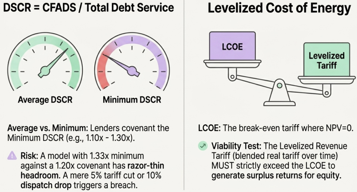
Average vs. Minimum DSCR

A model will report two DSCR figures. The average DSCR is the arithmetic mean across all years of the debt period – useful for an overall sense of the project’s debt-servicing ability. The minimum DSCR is the lowest single-year value across the entire debt period – this is what determines covenant compliance.

Lenders set a minimum DSCR covenant in the loan agreement. If the DSCR in any year falls below the covenant threshold, the project is technically in breach, which can trigger a range of remedies including cash sweeps, dividend restrictions, or in severe cases, acceleration of the entire loan. Typical covenant levels are 1.10× to 1.30× depending on risk profile.

DSCR Covenant Risk A model showing Minimum DSCR = 1.33× with an assumed covenant of 1.20× has a headroom of only 0.13×.  Test: What reduces DSCR by 0.13×?   – A 10% reduction in dispatched energy, OR   – A 5% tariff reduction, OR   – A 15% cost overrun in O&M, OR   – Any combination of the above  None of these is an extreme scenario. A model with thin DSCR headroom is a model that will breach its covenant under ordinary operational variability.

4.3 Payback Period

The payback period is the number of years required to recover the total investment from project cash flows. It is a simple, intuitive metric – but it must be interpreted carefully.

Two payback periods are commonly reported in infrastructure models:

• Payback from Commercial Operation Date (COD): How many years of operation are needed to recover total capital (debt + equity) from operating cash flows. This is typically 7–12 years for a well-structured hydropower project.
• Payback from Construction Start: Adds the construction period to the payback from COD. For a 5–7 year construction project, this is typically 12–19 years from the first rupee spent.

The payback period does not account for the time value of money (unlike IRR and NPV). It is most useful as a simple risk screen: a project with a 25-year payback on a 35-year licence is exposed to much more risk over its life than one with a 10-year payback. The sooner the investment is recovered, the less exposure to the tail risks discussed in Part 5.

4.4 Levelised Cost and Levelised Tariff

Two levelised metrics appear in sophisticated hydropower models, and they are frequently confused with each other.

Levelised Cost of Energy (LCOE)

The LCOE is the minimum tariff at which a project must sell energy in order to exactly recover all costs (capital, financing, O&M, replacement) over its life, discounted to present value. It is the break-even tariff.

LCOE Equation LCOE = NPV of All Lifetime Costs ÷ NPV of All Lifetime Energy (MWh)  Or equivalently, the tariff at which NPV = 0  Interpretation: If the project charges exactly its LCOE, investors earn zero economic profit (they recover their cost of capital, nothing more). Any tariff above LCOE generates value for equity investors.

Levelised Revenue Tariff

The levelised revenue tariff (sometimes called the levelised realised price) is the average effective tariff per kWh across all time periods and all tariff categories, weighted by the energy generated in each period and discounted to present value. It is not a policy-set number – it is a derived output that tells you the blended revenue rate actually captured by the project given its seasonal dispatch pattern.

The relationship between LCOE and the levelised revenue tariff tells you immediately whether the project is economically viable: if the levelised revenue tariff exceeds the LCOE, the project generates surplus returns. If it is below the LCOE, the project will fail to recover its costs even in the absence of any stress event.

Key Takeaway – Part 4 IRR tells you the return. DSCR tells you the resilience. Payback tells you the exposure. LCOE tells you the floor. Together, these four metrics give a complete financial portrait of a hydropower project – but only if each is calculated on consistent and verified assumptions. A high IRR built on an unchecked generation number or an unconfirmed concessional loan is not a return – it is an arithmetic fiction.

PART 5 – The Risks the Model Leaves Off the Page

Every financial model has a boundary. Inside the boundary, numbers are calculated with apparent precision – cash flows to four decimal places, IRRs to two. Outside the boundary are the things the model does not show: the events that cannot be easily parameterised, the structural risks that evolve over decades, and the scenarios that the developer prefers not to quantify. Part 5 is about finding the boundary and asking what is on the other side of it.

5.1 Physical Hazard Risks

Hydropower projects occupy some of the most physically hazardous environments on Earth: steep mountain watersheds subject to floods, earthquakes, and landslides; remote valleys with limited emergency access; rivers carrying enormous sediment loads. The financial model should quantify these risks, but in practice most models do not – or do so only in a footnote.

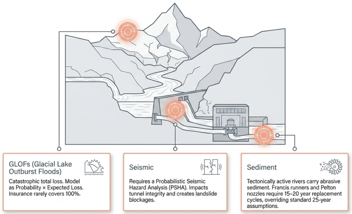
Glacial Lake Outburst Floods (GLOFs)

A Glacial Lake Outburst Flood occurs when a body of meltwater trapped behind a glacier or a moraine dam catastrophically releases, sending a massive flood surge downstream. The Himalayas, Andes, Hindu Kush, and other mountain ranges with retreating glaciers are all potential GLOF zones. Climate change is increasing both the number and volume of glacial lakes, and therefore the frequency and magnitude of potential outburst events.

The financial consequence of a GLOF striking a hydropower project can be total: complete destruction of diversion works, penstocks (the pressurised pipes carrying water to turbines), the powerhouse, and associated infrastructure. Reconstruction timelines are typically 2–5 years. The 2023 destruction of a large Himalayan hydropower project by a GLOF event – with losses exceeding USD 1.5 billion – demonstrated that this is not a theoretical risk.

GLOF Risk Assessment in a Financial Model A GLOF risk is correctly modelled as a probability-weighted expected loss:  Expected Annual Loss = Probability of GLOF per year × (Reconstruction Cost + Revenue Loss during outage)  Example:   Annual GLOF probability: 1%   Reconstruction cost: USD 500M   Revenue loss (3-year outage): USD 150M   Expected Annual Loss = 1% × USD 650M = USD 6.5M/year  This expected loss should either be reflected as a risk-adjusted reduction in NPV, or as a scenario (GLOF event in Year X) that shows the equity NPV at risk. The question for the insurer is: what portion of this USD 650M is actually recoverable under the policy?

GLOF-specific insurance riders are available in specialist reinsurance markets but may carry significant exclusions – particularly for downstream third-party claims. Establish clearly at model stage what the insurance recovery assumption is, and stress-test against a scenario where insurance pays only 50% of the loss.

Seismic Risk

Many of the world’s high-head hydropower sites are located in seismically active zones – the Himalayan fault system, the Ring of Fire in Southeast Asia and Latin America, the East African Rift. A major earthquake (Mw 7.0 or above) can damage tunnels, crack dams, destroy penstock alignments, and cause landslide blockages of access roads that extend reconstruction timelines by years.

Seismic risk should be assessed through a Probabilistic Seismic Hazard Analysis (PSHA) – a technical study that estimates the likelihood of ground accelerations of various magnitudes at the project site. The results feed into structural design standards and, for financial modelling purposes, into the probability and cost of seismic damage scenarios. Most large-scale infrastructure lenders require a PSHA as part of their due diligence.

Seismic Risk Gap If the financial model does not include a seismic scenario, ask: has a PSHA been conducted? If yes, what is the 1-in-500-year ground acceleration, and what would it cost to reconstruct critical structures damaged under that scenario? If no PSHA has been done, flag this as a mandatory lender requirement that will be identified in due diligence.

Sediment Load and Turbine Wear

Rivers in tectonically active mountain ranges carry very high sediment loads – the product of ongoing erosion from steep, geologically young slopes. Sediment concentration in the water passing through a hydropower turbine causes abrasive wear on the turbine components, reducing efficiency and eventually requiring replacement of expensive moving parts.

For technical reference, the main components subject to sediment wear in a hydropower turbine are:

• Runner: The rotating wheel of the turbine that converts water energy into rotational mechanical energy. In a Pelton turbine (used at very high heads, typically above 300m), the runner consists of buckets struck by high-velocity water jets. In a Francis turbine (medium to high head), the runner has curved vanes through which water flows. Runner replacement is the single most expensive maintenance item – typically USD 20–100M depending on turbine size.
• Nozzle and Jet Deflector (Pelton specific): The nozzle controls the water jet striking the Pelton runner. The jet deflector diverts the jet away from the runner during load rejection. Both are high-wear components in sediment-laden flows.
• Guide Vanes and Labyrinths (Francis specific): Control flow into the runner and seal between rotating and stationary parts. Subject to abrasive wear.
• Desilting Chambers / Settling Basins: Structures upstream of the turbines designed to settle out sediment before water enters the turbine. These require periodic flushing and maintenance; their effectiveness determines the sediment concentration reaching the turbines.

Sediment Wear Financial Impact Standard O&M budgets at 0.25–0.30% of build cost may be adequate for low-sediment rivers but insufficient for high-sediment mountain rivers. In the latter case, consider:  1. Runner replacement interval: Standard = 25 years. High-sediment = 15–20 years.    Earlier replacement increases NPV of capex by 20–35%.  2. Incremental O&M for desilting and wear: Add 0.05–0.10% of build cost per year as a dedicated sediment reserve.  3. Generation loss from efficiency degradation: In the year before major maintenance, a worn runner may operate at 3–7% below design efficiency, reducing revenue.

Cascade Dispatch Risk

Many hydropower rivers are not developed as single projects – they are developed in sequence along the same river, with multiple projects sharing the same waterway. This creates a cascade: water released from one project’s reservoir becomes the inflow to the next project downstream. In a regulated cascade, the entire system’s dispatch optimisation is shared – but in practice, individual project licences and different project owners mean that one project’s operational decisions can significantly affect another’s.

If a project upstream of yours is operated by a different entity – particularly a foreign entity with dispatch obligations to a different market (such as exporting to a neighbouring country) – its release schedule may be optimised for its own revenue, not yours. Your project’s inflow, head, and generation profile may become dependent on decisions made by an operator with different commercial interests.

Cascade Risk Checklist 1. Are there upstream or downstream projects on the same river whose operations materially affect your project’s inflow regime? 2. Is there a formal cascade coordination agreement between all project operators on that river? 3. If a cascade coordination agreement does not exist, what assumptions does the hydrological study make about upstream operating patterns? 4. What is the legal framework for resolving dispatch conflicts between cascade participants?  In the absence of a binding coordination agreement, cascade dependency should be modelled as a scenario in which inflow is reduced by 10–20% relative to the base hydrological assumption.

5.2 Single-Offtaker Risk in Emerging Markets

The vast majority of large hydropower projects in developing countries sell their entire output to a single national utility under a long-term PPA. This concentration creates a counterparty risk that is unique to infrastructure finance: the project’s revenue stream is only as secure as the financial health of one entity.

When a national utility is well-capitalised and operates in a well-regulated market with cost-reflective tariffs, this concentration is manageable. When the utility is financially stressed – carrying legacy debts, serving politically regulated tariffs below cost recovery, or cross-subsidising loss-making operations – the concentration becomes a genuine threat to project cash flows.

Offtaker Risk Indicator	What to Look For
Revenue adequacy	Does the utility’s end-user tariff cover its full cost of supply? If the utility is buying from you at 10 units/kWh but selling to consumers at 7 units/kWh and being subsidised by government, that subsidy is a policy risk.
Payment history	Has the utility been paying other project developers on time? Late payment to even one existing PPA is a warning signal.
Debt position	Is the utility carrying unsustainable debt from past loss-making operations or poorly-priced legacy PPAs?
Political exposure	Is the utility’s tariff-setting subject to political pressure that could prevent cost recovery?
Equity commitment	Is the utility simultaneously committed to contributing equity to multiple large projects while its profits are declining?

Sophisticated lenders – particularly multilateral development banks – will conduct a full financial health assessment of the offtaker as part of their due diligence. This assessment is sometimes more important than the project’s own financial model because the offtaker’s ability to pay is the ultimate source of debt service.

Offtaker Stress Scenario Model at minimum two offtaker stress scenarios:  Scenario A – Payment Delay: The offtaker pays 60 days late in every year from Year 5 onward. What is the impact on working capital requirements and DSCR?  Scenario B – Tariff Renegotiation: The offtaker (or its government principal) successfully renegotiates the tariff down by 10%. What is the minimum DSCR and equity IRR under this scenario?  A project that survives Scenario A comfortably and Scenario B with DSCR above covenant has genuine resilience. A project that breaches covenant in either scenario has a structural dependence on a single entity maintaining both its financial health and its contract obligations for 25+ years.

5.3 Currency Mismatch Risk

Currency mismatch arises when a project’s revenues and costs are denominated in different currencies. In most hydropower projects, revenue is collected in local currency (the tariff is set in local units) while a portion of costs – international debt service, imported equipment, and foreign technical staff – is in hard currency (USD, EUR, JPY). As the local currency depreciates, hard-currency costs rise in local-currency terms, squeezing the project’s margin.

Over a 25-year project life in an emerging market economy, the local currency may depreciate by 50–70% against the USD. This is not a scenario – it is a historical norm. Every year the model’s assumed depreciation rate diverges from the historical average, the gap between the modelled and the likely reality compounds.

Currency Mismatch Sensitivity Let x = hard currency cost as % of total annual costs Let d_assumed = FX depreciation assumed in model per year Let d_actual = historical average FX depreciation per year  Annual additional cost due to FX mismatch: Extra Cost % = x × (d_actual − d_assumed)  Example: 35% of costs are hard currency; model assumes 2.5%/yr; history shows 4.5%/yr: Extra Cost = 35% × (4.5% − 2.5%) = 0.70% of total costs per year  Over 25 years compounded, this is not trivial. Run the model at the historical average depreciation rate as the base case, not the optimistic rate.

5.4 Regulatory and Downstream Riparian Risk

Large hydropower projects in developing countries often attract the attention of regulatory bodies and international financial institutions that operate under environmental and social governance frameworks. One important but often overlooked requirement is the need to obtain the consent – or at minimum the formal consultation – of downstream riparian stakeholders.

Rivers do not respect political boundaries. A dam or diversion in one country affects water availability, flood dynamics, and ecosystem services downstream – potentially in a neighbouring country. Sophisticated infrastructure lenders, including multilateral development banks, apply lending frameworks that require evidence that downstream riparian interests have been consulted and that no material harm to downstream users will result.

Failure to manage this requirement can cause financing delays, withdrawal of lender support, or post-construction legal challenges that affect operations. This is not a theoretical risk – multiple large Himalayan and African hydropower projects have encountered significant financing delays due to unresolved downstream riparian concerns.

5.5 The Absence of Scenario Analysis – A Model is Not a Forecast

Perhaps the most important risk of all is not any single physical or financial hazard – it is the structural overconfidence built into a model that presents only one scenario. A financial model with a single base case is not a financial model. It is a best-case forecast dressed up with decimal-point precision.

A model presented to investors or lenders should always contain, at minimum:

• Base Case: The promoter’s central estimate with all current assumptions.
• Upside Case: A scenario in which key positive variables (hydrology, tariff escalation, construction timeline) outperform the base.
• Downside Case: A scenario with key negative variables – higher costs, lower dispatch, FX at historical rate.
• Financing Stress: What happens if the most favourable financing assumption (typically a concessional loan) is not available.
• Catastrophic Event: A single large-magnitude event (GLOF, seismic, offtaker default) to show equity NPV at risk.
• Combined Downside: Multiple negative factors simultaneously – not individually catastrophic, but collectively severe.

The Scenario Test When reviewing a model, ask: in how many of the scenarios presented does the project breach its DSCR covenant? In how many does the equity IRR fall below the required return?  If the answer is ‘none, because we only prepared a base case,’ the model has not been stress-tested. If the answer is ‘in two of six scenarios,’ you have a starting point for a real risk conversation.  A project that shows a convincing base case but cannot survive a single moderately adverse scenario is not a bankable project. It is a project that needs its assumptions re-examined.

Key Takeaway – Part 5 The risks in the model are the ones the developer chose to put there. The risks that matter most are often the ones they chose not to. Read the assumptions page as carefully as the results page. Look for what is absent. GLOF, seismic, cascade, offtaker stress, currency mismatch, and the absence of scenario analysis are the most common silences in hydropower financial models. Each silence has a price.

CLOSING – Putting It All Together

Across all five parts, certain themes recur:

Theme	The Core Question
What is confirmed vs. assumed?	Every assumption in a financial model sits on a spectrum from ‘legally binding and documented’ to ‘optimistic working assumption.’ Know where each critical assumption sits before trusting the output.
What happens when the base case is wrong?	A model without scenario analysis is a wish, not an analysis. The value of a financial model is not in its base case – it is in its ability to show you how much you can lose and under what conditions.
Who bears the risk?	Debt, equity, government, and offtaker each bear different risks under different conditions. Understanding the risk allocation – and whether it matches each party’s capacity to absorb it – is the purpose of the financing structure.
What does the model not show?	Physical hazards, regulatory changes, cascade interactions, and offtaker stress are routinely absent from financial models. A good reviewer knows how to find these absences and asks for them to be filled.
Is the timeline realistic?	Construction timelines, financial close dates, and COD are the most consistently optimistic numbers in infrastructure models. Treat them as aspirations until the critical path of agreements and licences confirms them.

Reading a hydropower financial model well is not primarily a mathematical skill. It is a judgement skill – the ability to ask which numbers matter most, which assumptions are load-bearing, and where the model’s map ends and unexplored territory begins. The equations and benchmarks in this guide are tools for that judgement, not substitutes for it.

Series: Hydro Series